Diffusion Decoder based Compression
Published:
I’m always super interested in expanding the fronteir of learned compression. The current methods we use are derived from VAEs (equivalence shown here) and use GANs to improve preceptual quality but in this blog I explore how diffusion models could be used for compression.
The feasibility of any method we explore in a learned compression pipeline hinges on the complexity of that method. Since decode and sometime encode are performed on battery constrained edge devices, the scope of a new method to add compute is very limited, often 1-2KMACs/px. As a result training time improvements are favoured over encode/decode. In this blog though, we’ll go against this advice and augument our deocoder with a denoising diffusion encoder.
Intro to Diffusion Models
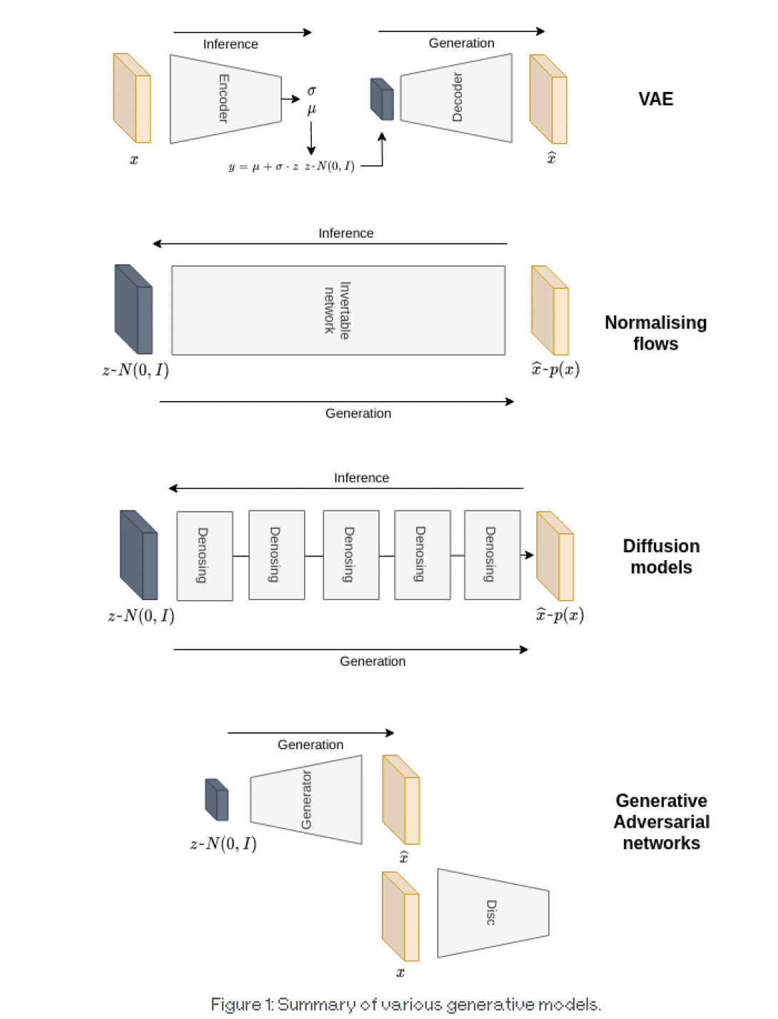
Before we dive into diffusion models, let’s summarise the main methods for generating from a distribution currently available to us, and see how diffusion models look compared to them. This is shown in Figure 1.
The forward process
The forward step in a diffusion model consists of adding small amounts of Gaussian noise to our image (which is sampled from our data distribution), until it looks like a Gaussian sample from \(N(0, I)\). We define a number of steps we want to achieve this transition in, and at each step, we add noise with a variance we pre-set (we call this the variance schedule). Since each transition depend only on the present state, the forward process is Markovian and can be written as:
\[q(x_t | x_{t-1}) = N\left(x_t; \sqrt{1-\beta_t}x_{t-1}, \beta_t I\right)\] \[q(x_{1:T} | x_0) = \prod_{t=1}^T q(x_t | x_{t-1})\]Here, \(\beta_t\) is our variance at time step \(t\). As well as adding noise, we also scale down the previous sample by \(\sqrt{1-\beta_t}\) which is required if we are to bound the variance of \(x_t\) in the limited of a standard normal. This will be graphically shown later.
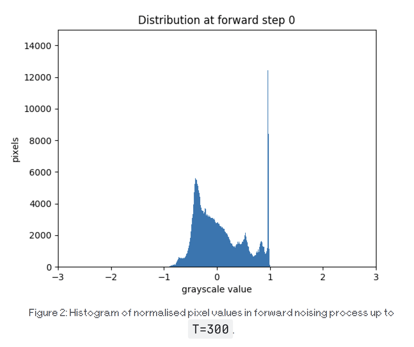
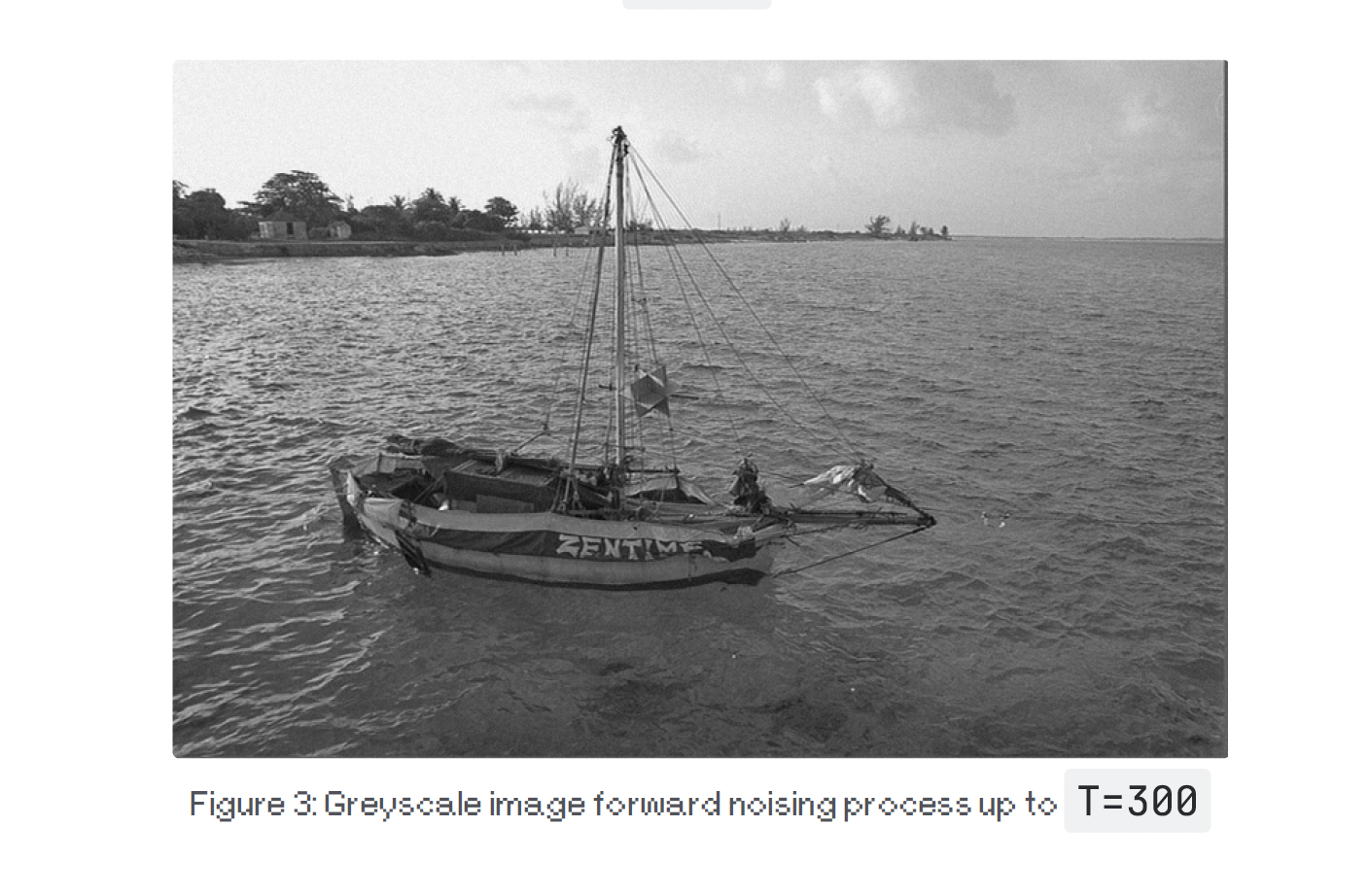
Now, let’s see what this means in practice. Let’s take an image from the Kodak dataset, and define a variance schedule over \(T = 1000\) steps, starting at \(\beta = 10^{-4}\) and ending at \(\beta = 0.02\). Figures 2 and 3 below show a greay scale image and it’s grey value pixel distribution.
Let’s have a closer look at what is actually happening in the forward noising process and some of its useful properties. Essentially, at each step \(t\) we are adding small amounts of Gaussian noise with a particular variance to the sample from the previous step, \(t-1\), while scaling it down with \(\sqrt{1-\beta_t}\). To help with notation, let’s write \(\beta_t = 1 - \alpha_t\). Figure 4 shows the forward step diagrammatically.
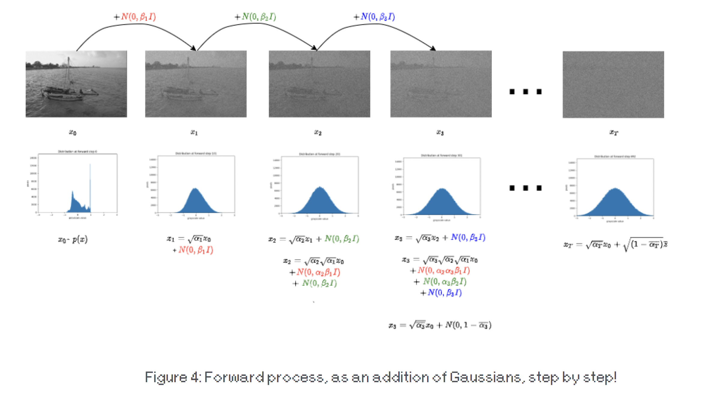
Figure 4 shows that at any point in the forward process, we can break down the current sample \(x_t\) into two terms:
The initial data sample we are noising (\(x_0\) from \(p_x\)) and a cumulative product of scaling coefficients for \(x_0\), square root of \(\bar{\alpha}_t = \prod_{s=1}^t \alpha_s\) (which depends on the time step we are on and the self-defined variance schedule)
A set of mean-zero Gaussian with different scales where the scales depend on the current time step and self-defined variance schedule. Using the properties of Gaussians, we can combine all these zero-mean Gaussians into one Gaussian with a particular variance, which is just the addition of the variance of all the Gaussians up to the point and takes the form \(1 - \bar{\alpha}_t\). A simple derivation of this is shown later.
Scaling x
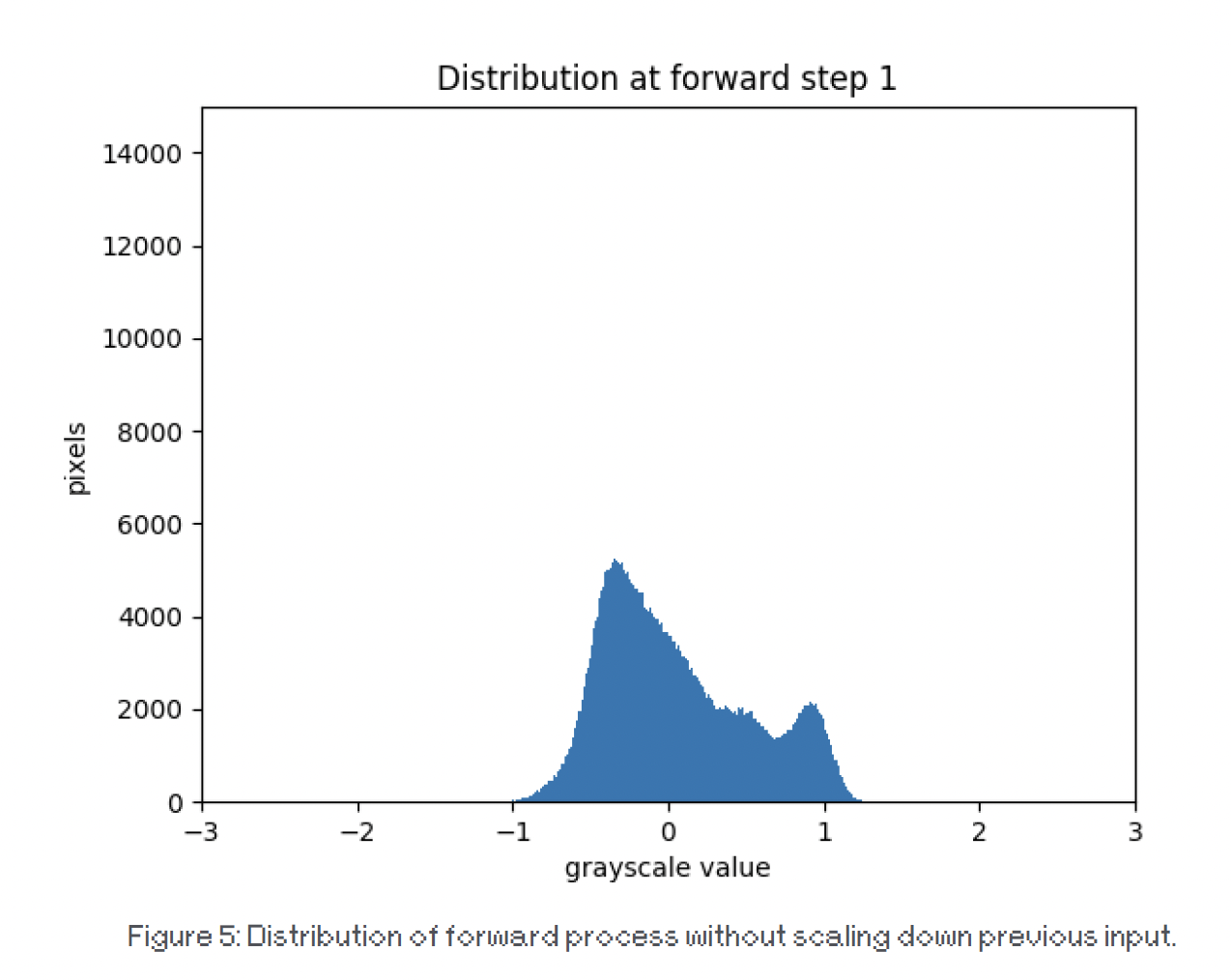
Why do we need to scale down the previous input \(x_{t-1}\) at each step by the current variance? Well, let’s have a look at what happens if we don’t. Figure 5 shows the same process as Figure 4, but where the \(x_{t-1}\) is not scaled down by \(\sqrt{1-\beta_t}\). We observe that the variance of the distribution continues to grow and its tails become fatter, which means it is not an \(N(0, I)\).
Sampling \(x_t\) at an arbitrary time step \(t\)
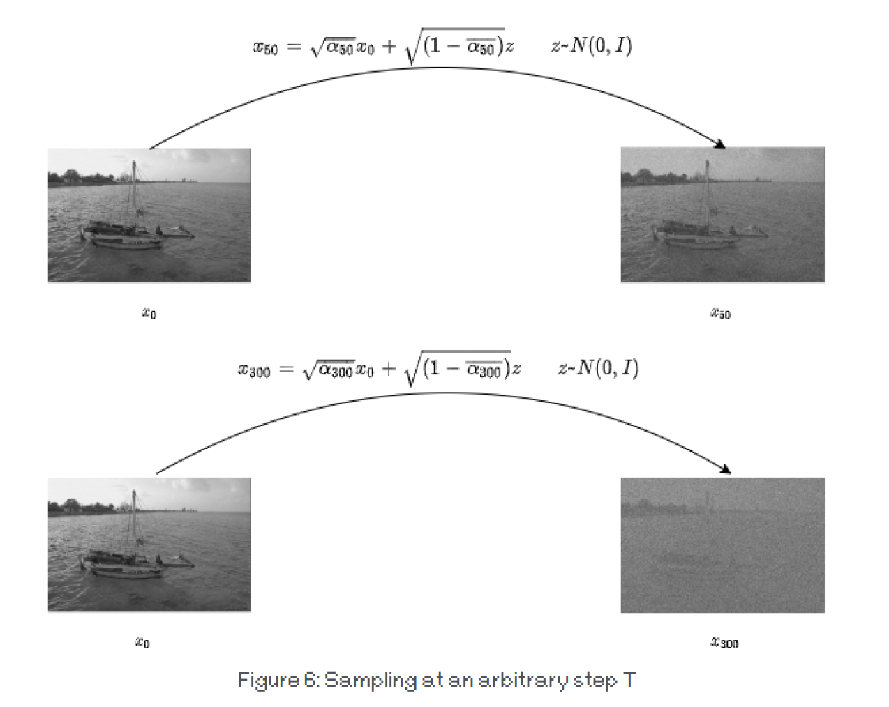
Since we are adding a lot of Gaussians to a sample, this affords us the nice properties Gaussians bring with them. One useful property we can extract from this is the ability to sample a noisy \(x_t\) at any time step (without having to go through the entire forward process up to that point), given an \(x_0\). This is because we define the variance schedule and therefore, at any time steps, we know all the Gaussian samples that were added to \(x_0\) to get that particular noisy \(x_t\). Figure 4 already shows this, but here we provide more detail.
\[t = 0:\] \[x_0 \sim p_x(x)\] \[t = 1:\] \[x_1 = \sqrt{1-\beta_1}x_0 + N(0, \beta_1 I)\] \[= \sqrt{1-\beta_1}x_0 + 0 + \sqrt{\beta_1}z_1\] \[t = 2:\] \[x_2 = \sqrt{1-\beta_2}x_1 + N(0, \beta_2 I)\] \[= \sqrt{1-\beta_2}\left(\sqrt{1-\beta_1}x_0 + \sqrt{\beta_1}z_1\right) + \sqrt{\beta_2}z_2\] \[= \sqrt{\alpha_2}\left(\sqrt{\alpha_1}x_0 + \sqrt{1-\alpha_1}z_1\right) + \sqrt{1-\alpha_2}z_2\] \[= \sqrt{\alpha_2\alpha_1}x_0 + \sqrt{(1-\alpha_1)\alpha_2 + (1-\alpha_2)}\bar{z}\] \[= \sqrt{\bar{\alpha}_2}x_0 + \sqrt{(1-\bar{\alpha}_2)}\bar{z}\]For any \(t\):
\[x_t = \sqrt{\bar{\alpha}_t}x_0 + \sqrt{(1-\bar{\alpha}_t)}\bar{z}\]Here, \(z\) is a sample from a standard normal. The figure below demonstrates how we can jump from \(x_0\) directly to \(x_{50}\) and \(x_{100}\) though combining all the variances of the Gaussian in the chain up to those points. This is an extremely useful property and will help us in training as we shall see later.
The reverse process
The true reverse process of our posterior is written as:
\[p_\theta(x_{t-1} | x_t) = N(x_{t-1}; \mu_\theta(x_t, t), \Sigma_\theta(x_t, t)I).\]Like variational inference, we define an approximate distribution for our forward process \(q(x_{t-1} \mid x_t)\), and close the gap between the two using KL-divergence.
\(q(x_{t-1} \mid x_t)\) is generally intractable; however, it can be shown to be tractable when conditioned on \(x_0\). This results in the following formulation of what we call the forward process posterior:
\[q(x_{t-1} | x_t, x_0) = \mathcal{N}\left( \mu_{\text{post}}, \tilde{\beta}_t I \right)\]where the posterior mean is:
\[\mu_{\text{post}} = \frac{\sqrt{\bar{\alpha}_{t-1}}\beta_t}{1-\bar{\alpha}_t}x_0 + \frac{\sqrt{\alpha_t}(1-\bar{\alpha}_{t-1})}{1-\bar{\alpha}_t}x_t\] \[\tilde{\beta}_t = \frac{\beta_t(1-\bar{\alpha}_{t-1})}{1-\bar{\alpha}_t}\]This can be derived with (2.116) in Bishop’s book. Therefore, if we can predict our posterior mean \(\mu_{\text{post}}\) and our variance (which we can easily be computed as all terms are always known), we should be able to sample from our reverse posterior \(q(x_{t-1} | x_t, x_0)\).
If we have a look at this mean, during the reverse/sampling process, we know \(\bar{\alpha}\) and \(\beta\) as these are self-defined. \(x_t\) is the current step we are on, which we know too (since we start with a sample form \(N(0, I)\)). The only term we do not know at sampling time is \(x_0\). This is what we need a neural network to help us predict. We can train a network \(f_\theta(x_t, t)\) to directly predict this, given \(x_t\) and \(t\) as inputs, however, this is empirically shown not to work too well, and a better method is to do the following:
We know from the forward process that:
\[x_t = \sqrt{\bar{\alpha}_t}x_0 + \sqrt{(1-\bar{\alpha}_t)}\varepsilon\]where \(\varepsilon \sim N(0, I)\) which we can rearrange to get an approximation of \(x_0\), say \(\tilde{x}_0\):
\[\tilde{x}_0 = \frac{1}{\sqrt{\bar{\alpha}_t}}\left(x_t + \sqrt{1-\bar{\alpha}_t}\varepsilon\right)\]We can plug this formula in for \(x_0\) in the forward process posterior definition to obtain the reverse sampling step:
\[x_{t-1} = \frac{1}{\sqrt{\alpha_t}}\left(x_t - \frac{\beta_t}{\sqrt{1-\alpha_t}}\varepsilon\right) + \tilde{\beta}_t z, \quad z \sim N(0, I)\]This leaves us with the unknown noise sample \(\varepsilon\) from a standard normal which we need to predict; all other terms are known. We can define a neural network to predict this term:
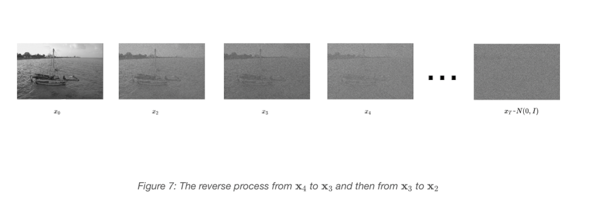
\[\varepsilon \approx f_\theta(x_t, t) = \varepsilon_\theta\]Once we have estimated \(\varepsilon\), we can compute \(\tilde{x}_0\), after which we can predict \(\tilde{\mu}\) and sample the \(x_{t-1}\). Then we can repeat this process, until we get to \(x_0\) which is our sample from the distribution. Figure 7 shows this process in steps in the order they are performed during sampling, starting at \(x_4\) and predicting \(x_3\) and then \(x_2\).
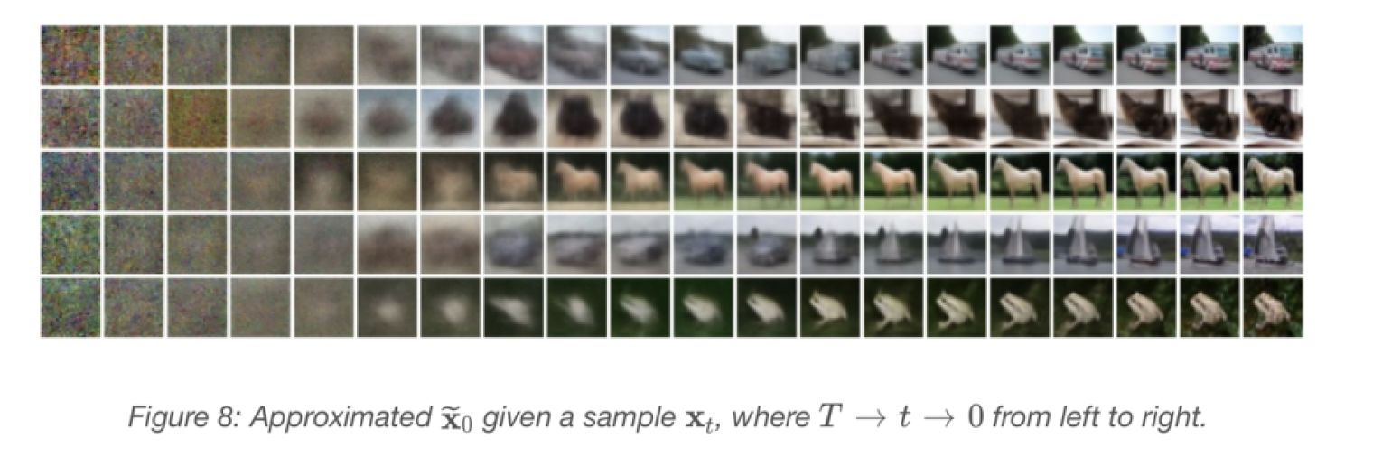
What does \(\tilde{x}_0\) look like at each time step? That depends on where you are; if you are quite early in the chain, it looks like noise with some structure. If you are close to the end of the chain, it almost looks like an image. An example is shown in Figure 8, taken from the DDPM paper.
Training
The loss function is a maximisation problem of the variational lower bound on the log-likelihood of the data:
\[\mathbb{E}_q(x_0)[\log p_\theta(x_0)] \geq -\mathbb{E}_q(x_0)[\log q(x_{1:T} | x_0) - \log p_\theta(x_{0:T})] = -\mathcal{L}\]This can be reduced to a sum of KL-divergences between \(q(x_{t-1} \mid x_t, x_0)\) and \(p_\theta(x_{t-1} \mid x_t)\). Since both are Gaussian, this is just a KL between two Gaussians. Working through this, we can end up with a simplified loss term (we need to drop some scaling constants that arise when we do the KL between the Gaussians), corresponding to a weighted variational lower bound:
\[\mathcal{L}_{\text{simple}} = \mathbb{E}_{x_0, \varepsilon}\left(\|\varepsilon - \varepsilon_\theta(x_t, t)\|_2^2\right)\]This is the simplified objective we can use to train our denoising function \(\varepsilon_\theta\), which is generally selected to be some sort of U-Net architecture. What this denoising function learns during training is the noise that was added to samples from the dataset to noise them. Once it is fully trained, it can then be used to remove that noise. The training process is then extremely simple and is performed as below:
We select a random time step \(t\)
We sample an instance of noise: \(\varepsilon \sim N(0, I)\)
We generate the noisy sample \(x_t\) at this time step using the sampled noise \(\varepsilon\) and variance schedule (see forward process section)
We feed this \(t\) and \(x_t\) to our denoising function \(\varepsilon_\theta(x_t, t)\) to approximate \(\varepsilon\)
We use an L2-metric to compute a loss between \(\varepsilon\) and \(\varepsilon_\theta\)
Conditional compression denoising decoder
Is there a way we could use diffusion models in our compression pipeline? Can they be used for explicit likelihood or implicit distribution matching?
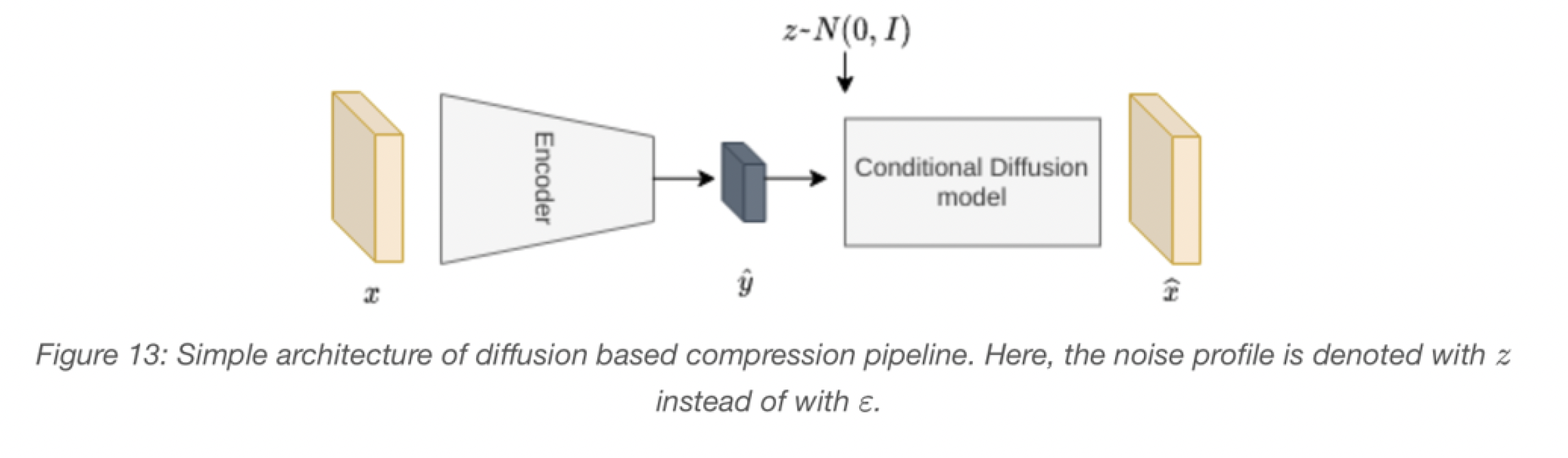
An immediate idea would be to replace our decoder with a conditional diffusion model where we condition the diffusion process on the quantised latent space. This would enable conditional image generation allowing rate and distortion training as usual.
There are a few changes that we would need to consider for the pipeline. Let’s break them down into architecture, training and inference.
Architecture:
Until the decoder, our architecture can remain the same, however, we would then need to upsample our quantised latent space to the image scale (diffusion models work on the image scale).
We need to define a function \(\varepsilon_\theta\), which empirically is showed to work best as a U-Net architecture. The input of the U-Net will need to be a noise vector concatenated with an upsampled latent space.
The training:
The training function we minimise now becomes:
\[L = \mathbb{E}_{x_0 \sim p(x_0)} \left( \mathbb{E}_{\varepsilon \sim N(0,I)} \left( \|\varepsilon - \varepsilon_\theta(x_t, t, \hat{y}_{us})\|_2^2 \right) + R \right)\]where \(\varepsilon\theta\) has an additional input to force it to be conditional.
The inference:
The encoding works exactly the same, but the decoding differs. After the \(\hat{y}\) is produced, we sample a \(\varepsilon\), and perform the computation as shown in Figure 7 for some number of steps to get out final output \(\hat{x}\).
I ran the above model and it produced competitive results on the first iteration. I have high hopes for the compression performance, but the largest concern is with execution time. We’d need to see a lot more algorithmic progress in diffusion decoders to enable efficient decoding.